
Hierarchical Clustering in Machine Learning : A Comprehensive Guide
Introduction
Clustering is a cornerstone of unsupervised machine learning, enabling the grouping of similar data points to uncover patterns or structures within unlabeled datasets. Among clustering techniques, hierarchical clustering stands out for its ability to create a hierarchy of clusters, offering a detailed view of data relationships through a tree-like structure known as a dendrogram. This method is particularly valuable when the number of clusters is unknown, as it does not require pre-specifying cluster counts, unlike K-means clustering.
In this comprehensive guide, tailored for students and aspiring data scientists, we will explore hierarchical clustering in depth. We will cover its theoretical foundations, step-by-step processes, practical examples, and real-world applications. By the end, you will have a thorough understanding of how to apply hierarchical clustering and interpret its results effectively.
What is Hierarchical Clustering?
Hierarchical clustering is an unsupervised machine learning algorithm that organizes data points into clusters based on their similarity or dissimilarity. It constructs a hierarchy of clusters, represented as a dendrogram, which visually depicts how data points are grouped at various levels of granularity. This hierarchy allows analysts to explore data relationships and choose the number of clusters that best suits their needs.
There are two primary approaches to hierarchical clustering:
- Agglomerative (Bottom-Up):
- Each data point begins as an individual cluster.
- The algorithm iteratively merges the closest pairs of clusters until all points are combined into a single cluster.
- This approach is more commonly used due to its computational efficiency and interpretability.
- Divisive (Top-Down):
- All data points start in a single cluster.
- The algorithm recursively splits clusters into smaller ones until each point is its own cluster.
- This method is less common due to its higher computational complexity.
For this guide, we will focus on the agglomerative approach, as it is widely adopted and easier to implement.
How Does Agglomerative Hierarchical Clustering Work?
The agglomerative hierarchical clustering algorithm follows a systematic process to build the cluster hierarchy. Below is a step-by-step explanation:
- Initialize Clusters:
- Treat each data point as a separate cluster. For a dataset with n n n points, there are initially n n n clusters.
- Compute Distances:
- Calculate the distance (dissimilarity) between all pairs of clusters using a chosen distance metric, such as Euclidean or Manhattan distance.
- Merge Closest Clusters:
- Identify the pair of clusters with the smallest distance and merge them into a single cluster, reducing the total number of clusters by one.
- Update Distance Matrix:
- Recalculate distances between the new cluster and all remaining clusters, using a linkage method to define how distances are computed between clusters.
- Repeat:
- Continue merging clusters and updating the distance matrix until all data points are combined into a single cluster.
- Construct Dendrogram:
- Represent the merging process as a dendrogram, where the x-axis lists data points, and the y-axis indicates the distance at which clusters are merged.
This process results in a hierarchical structure that can be analyzed to determine the optimal number of clusters.
Key Components: Distance Metrics and Linkage Methods
To perform hierarchical clustering, two critical decisions must be made: the distance metric to measure dissimilarity between data points and the linkage method to calculate distances between clusters.
Distance Metrics
Distance metrics quantify the dissimilarity between data points. Common metrics include:
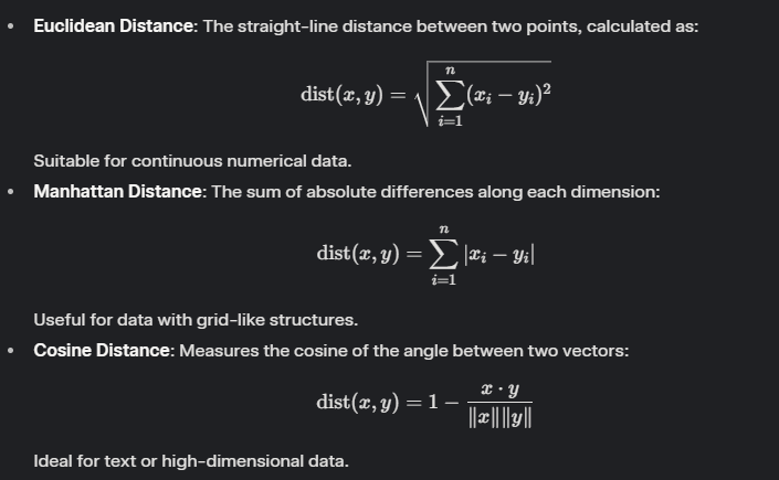
The choice of distance metric depends on the data type and the problem domain. For example, Euclidean distance is effective for spatial data, while cosine distance is preferred for text analysis.
Linkage Methods
Linkage methods determine how the distance between two clusters is calculated. The most common methods are:
Linkage methods determine how the distance between two clusters is calculated. The most common methods are:
- Single Linkage: The distance between two clusters is the minimum distance between any two points in the clusters.
- Advantages: Detects non-spherical clusters.
- Disadvantages: Prone to “chaining,” where clusters merge prematurely.
- Complete Linkage: The distance is the maximum distance between any two points in the clusters.
- Advantages: Produces compact clusters, less sensitive to outliers.
- Disadvantages: May favor elongated clusters.
- Average Linkage: The distance is the average of all pairwise distances between points in the two clusters.
- Advantages: Balances single and complete linkage, suitable for medium-sized datasets.
- Disadvantages: Computationally intensive for large datasets.
- Ward’s Method: Minimizes the increase in total within-cluster variance when merging clusters.
- Advantages: Produces spherical, compact clusters.
- Disadvantages: Computationally expensive, assumes clusters are of similar size.
The linkage method significantly influences the shape and structure of the resulting clusters. Ward’s method is often a robust default choice for many applications.
Dendrograms: Visualizing the Hierarchy
A dendrogram is a tree-like diagram that illustrates the hierarchical clustering process. Key features include:
- Leaves: Represent individual data points at the bottom of the diagram.
- Branches: Indicate the merging of clusters, with horizontal lines showing cluster unions.
- Height: Reflects the distance (dissimilarity) at which clusters are merged, with taller branches indicating greater dissimilarity.
- Cutting the Dendrogram: To obtain a specific number of clusters, a horizontal line is drawn across the dendrogram. The number of vertical lines intersected by this cut determines the number of clusters.
For example, cutting at a low height results in many small clusters, while cutting at a high height yields fewer, larger clusters. The dendrogram is a powerful tool for visualizing data relationships and selecting an appropriate number of clusters.
Example 1: Clustering Fruits by Weight
To illustrate hierarchical clustering, consider a simple dataset of four fruits with the following weights:
| Fruit | Weight (g) |
|---|---|
| Apple | 100 |
| Banana | 120 |
| Cherry | 50 |
| Grape | 30 |
We will use the absolute difference (Manhattan distance in one dimension) as the distance metric and average linkage for merging clusters.
Step-by-Step Process
- Initial Distance Matrix:
Calculate the absolute differences between all pairs of fruits:
- Dist(Apple, Banana) = |100 – 120| = 20
- Dist(Apple, Cherry) = |100 – 50| = 50
- Dist(Apple, Grape) = |100 – 30| = 70
- Dist(Banana, Cherry) = |120 – 50| = 70
- Dist(Banana, Grape) = |120 – 30| = 90
- Dist(Cherry, Grape) = |50 – 30| = 20 The distance matrix is: Apple Banana Cherry Grape Apple 0 20 50 70 Banana 20 0 70 90 Cherry 50 70 0 20 Grape 70 90 20 0
- First Merge:
The smallest distance is between Cherry and Grape (20). Merge them into a cluster {Cherry, Grape}, with an average weight of (50 + 30) / 2 = 40g. - Update Distance Matrix:
Calculate distances between the new cluster and remaining points:
- Dist({Cherry, Grape}, Apple) = |40 – 100| = 60
- Dist({Cherry, Grape}, Banana) = |40 – 120| = 80
- Dist(Apple, Banana) = 20 (unchanged) Updated matrix: Apple Banana {Cherry, Grape} Apple 0 20 60 Banana 20 0 80 {Cherry, Grape} 60 80 0
- Second Merge:
The smallest distance is between Apple and Banana (20). Merge them into {Apple, Banana}, with an average weight of (100 + 120) / 2 = 110g. - Final Merge:
Calculate the distance between {Apple, Banana} and {Cherry, Grape}:
- Dist({Apple, Banana}, {Cherry, Grape}) = |110 – 40| = 70
Merge them into a single cluster: {Apple, Banana, Cherry, Grape}.
Dendrogram Representation
The hierarchy can be described as:
- Step 1: Merge Cherry and Grape at distance 20.
- Step 2: Merge Apple and Banana at distance 20.
- Step 3: Merge {Apple, Banana} and {Cherry, Grape} at distance 70.
In a dendrogram, Cherry and Grape would be connected at a height of 20, Apple and Banana at a height of 20, and the final merge at a height of 70. This visualization helps identify natural groupings, such as lighter fruits (Cherry, Grape) versus heavier fruits (Apple, Banana).
Example 2: Real-World Application with Loan Data
To demonstrate hierarchical clustering in a practical context, consider a loan dataset with features such as credit score, loan amount, interest rate, and income. This example draws inspiration from a loan dataset analysis, where the goal is to segment borrowers into risk-based groups.
Step-by-Step Process
- Data Preprocessing:
- Remove Missing Values: Ensure the dataset is complete by excluding rows with missing entries.
- Handle Outliers: Use the Interquartile Range (IQR) method to identify and remove outliers, ensuring robust clustering.
- Scale Features: Apply standardization (e.g., using StandardScaler) to normalize features, as hierarchical clustering is sensitive to scale differences.
- Select Distance Metric and Linkage Method:
- Choose Euclidean distance for numerical features like credit score and loan amount.
- Test multiple linkage methods (e.g., complete, average, Ward’s) to identify the most meaningful clusters.
- Apply Hierarchical Clustering: Use Python’s scikit-learn library to perform clustering. Below is a sample code snippet:
from sklearn.cluster import AgglomerativeClustering
from sklearn.preprocessing import StandardScaler
import numpy as np

# Assume 'X' is the preprocessed loan dataset
scaler = StandardScaler()
X_scaled = scaler.fit_transform(X)

# Apply hierarchical clustering with Ward's method
hc = AgglomerativeClustering(n_clusters=3, linkage='ward')
labels = hc.fit_predict(X_scaled)- Visualize the Dendrogram:
Use SciPy to generate a dendrogram for visual analysis:
from scipy.cluster.hierarchy import linkage, dendrogram
import matplotlib.pyplot as plt

# Perform linkage
Z = linkage(X_scaled, method='ward')

# Plot dendrogram
plt.figure(figsize=(10, 7))
dendrogram(Z)
plt.title('Hierarchical Clustering Dendrogram')
plt.xlabel('Sample Index')
plt.ylabel('Distance')
plt.show()- Interpret Clusters:
- Cut the dendrogram to obtain, for example, three clusters.
- Analyze the mean feature values for each cluster to interpret their characteristics:
- Cluster 1: High credit scores, low loan amounts (low-risk borrowers).
- Cluster 2: Low credit scores, high loan amounts (high-risk borrowers).
- Cluster 3: Moderate credit scores, variable loan amounts (medium-risk borrowers).
Sample Python Code for Visualization
To further illustrate, here is a complete example using synthetic data to demonstrate hierarchical clustering:
import numpy as np
from sklearn.datasets import make_blobs
from scipy.cluster.hierarchy import linkage, dendrogram
import matplotlib.pyplot as plt

# Generate synthetic data with 3 clusters
X, _ = make_blobs(n_samples=100, centers=3, cluster_std=0.60, random_state=0)

# Perform hierarchical clustering
Z = linkage(X, method='ward')

# Plot dendrogram
plt.figure(figsize=(10, 7))
plt.title('Hierarchical Clustering Dendrogram')
plt.xlabel('Sample Index')
plt.ylabel('Distance')
dendrogram(Z)
plt.show()

# Plot clusters
from sklearn.cluster import AgglomerativeClustering
hc = AgglomerativeClustering(n_clusters=3, linkage='ward')
labels = hc.fit_predict(X)

plt.figure(figsize=(8, 6))
plt.scatter(X[:, 0], X[:, 1], c=labels, cmap='viridis')
plt.title('Hierarchical Clustering Results')
plt.xlabel('Feature 1')
plt.ylabel('Feature 2')
plt.show()
This code generates a synthetic dataset with three clusters, performs hierarchical clustering, and visualizes both the dendrogram and the resulting clusters in a scatter plot.
Applications of Hierarchical Clustering
Hierarchical clustering is applied across diverse domains due to its flexibility and interpretability. Key applications include:
- Biology: Clustering gene expression data to identify co-expressed genes or constructing taxonomic hierarchies.
- Marketing: Segmenting customers based on purchasing behavior for targeted marketing strategies.
- Image Processing: Grouping similar pixels for image segmentation or object recognition.
- Social Network Analysis: Identifying communities or groups within social networks based on interaction patterns.
These applications highlight the versatility of hierarchical clustering in uncovering meaningful patterns in complex datasets.
Advantages and Disadvantages
Advantages
- No Predefined Cluster Count: Unlike K-means, hierarchical clustering does not require specifying the number of clusters in advance.
- Hierarchical Representation: The dendrogram provides a clear visualization of cluster relationships at multiple levels.
- Handles Nested Clusters: Effective for datasets with subclusters or hierarchical structures.
- Robust to Noise: Certain linkage methods, like complete linkage, are less sensitive to outliers.
Disadvantages
- Computational Complexity: The algorithm has a time complexity of O(n²) or O(n³), making it less scalable for large datasets.
- Sensitivity to Parameters: Results depend heavily on the choice of distance metric and linkage method.
- Difficulty with Large Datasets: Memory and computational requirements can be prohibitive for very large datasets.
- Interpretation Challenges: Dendrograms for complex datasets may be difficult to interpret without domain expertise.
Comparison with Other Clustering Techniques
To provide context, let’s compare hierarchical clustering with other common clustering methods:
| Method | Key Characteristics | Advantages | Disadvantages |
|---|---|---|---|
| Hierarchical | Builds a hierarchy of clusters, visualized as a dendrogram. | No need to specify cluster count, interpretable hierarchy. | Computationally expensive, sensitive to parameters. |
| K-means | Partitions data into K clusters based on centroids. | Fast, efficient for large datasets. | Requires predefined K, sensitive to outliers. |
| DBSCAN | Groups points based on density, automatically determines cluster count. | Handles noise, detects arbitrary shapes. | Requires tuning of parameters, less effective for varying densities. |
| Gaussian Mixture | Uses probabilistic models to assign points to clusters. | Flexible for complex shapes, soft clustering. | Computationally intensive, requires model selection. |
Hierarchical clustering is particularly suited for exploratory analysis and datasets with hierarchical structures, but it may not be the best choice for very large datasets where K-means or DBSCAN might be more efficient.
Handling Special Cases
- Categorical Data: Convert categorical variables to numerical formats using techniques like one-hot encoding or ordinal encoding before applying hierarchical clustering.
- Large Datasets: For scalability, consider sampling the data or using faster linkage methods like single linkage, though this may compromise cluster quality.
- Outliers: Preprocess data to remove or mitigate outliers, as they can significantly affect clustering results, especially with single linkage.
Conclusion
Hierarchical clustering is a powerful and flexible method for grouping similar data points in unsupervised machine learning. Its ability to create a hierarchy of clusters, visualized through a dendrogram, makes it an excellent tool for exploratory data analysis. By understanding the roles of distance metrics, linkage methods, and dendrograms, students and practitioners can apply hierarchical clustering to diverse problems, from customer segmentation to biological classification.