
Credit Card Transactions Analysis
This guide walks you through credit card transactions analysis using Python’s Pandas library, with clear visualizations from Matplotlib and Seaborn. For example, you’ll learn to clean data, detect fraud, and uncover customer behavior trends in a credit card transactions dataset. Additionally, explore related topics in our Pandas Data Cleaning Guide or read about fraud detection in this article on financial fraud. This step-by-step tutorial simplifies credit card transactions analysis for data analysts and financial professionals.
Why Credit Card Transactions Analysis Matters
Analyzing credit card transactions helps financial companies spot fraud, understand customer habits, and make data-driven decisions. This tutorial uses a dataset, credit_card_transactions.csv, to guide you through credit card transactions analysis. Moreover, you’ll merge it with customer_info.csv to explore demographic trends. The goal is to clean, manipulate, and analyze data for actionable insights, such as fraud detection and customer behavior patterns.
Objective
The objective is to develop expertise in:
- Data Cleaning: Handling missing values and ensuring data consistency.
- Data Manipulation: Creating new features and categorizing data.
- Data Analysis: Aggregating data to uncover trends and patterns.
- Fraud Detection: Identifying suspicious transaction patterns.
- Data Visualization: Presenting insights through charts and heatmaps.
We will work with the credit_card_transactions.csv dataset and an additional customer_info.csv dataset to perform a thorough analysis.
Problem Statement
As a data analyst for a financial company, the task is to analyze credit card transaction data to provide insights for decision-making. The dataset contains detailed transaction information, and the analysis will focus on trends, anomalies, and customer behavior to enhance fraud detection and business strategies.
Dataset Overview – Credit Card Transactions Analysis
The credit_card_transactions.csv dataset includes : Download DataSet
- Transaction_ID: Integer, unique transaction identifier.
- Customer_ID: Integer, unique customer identifier.
- Transaction_Date: String, date of transaction (YYYY-MM-DD).
- Transaction_Type: String, type of transaction (e.g., Online, POS, ATM).
- Merchant: String, name of the merchant.
- Category: String, purchase category (e.g., Groceries, Electronics, Travel).
- Amount: Float, transaction amount in USD.
- Payment_Mode: String, payment method (e.g., Credit Card, Debit Card).
- Transaction_Status: String, status (Approved, Declined, Pending).
- Location: String, city where the transaction occurred.
The customer_info.csv dataset includes : Download DataSet
- Customer_ID: Integer, unique customer identifier.
- Age: Integer, customer’s age.
- Gender: String, customer’s gender.
- Account_Status: String, customer’s account status.
Step-by-Step Guide to Credit Card Transactions Analysis
Below is a Python script with detailed explanations for each step of credit card transactions analysis. The code addresses data cleaning, filtering, feature engineering, aggregation, fraud detection, and visualization.
Step 1: Data Exploration and Cleaning
Objective: Load the dataset, inspect its structure, handle missing values, and prepare the data for analysis.
Code
import pandas as pd
import numpy as np
import matplotlib.pyplot as plt
import seaborn as sns
from datetime import datetime, timedelta

# Load the dataset
df = pd.read_csv('credit_card_transactions.csv')

# Display first 5 rows
print("Step 1.1: First 5 rows of the dataset:")
print(df.head())

# Check shape, column names, and summary statistics
print("\nStep 1.2: Dataset Shape:", df.shape)
print("\nStep 1.3: Column Names:", df.columns.tolist())
print("\nStep 1.4: Summary Statistics:")
print(df.describe(include='all'))

# Identify missing values
print("\nStep 1.5: Missing Values:")
print(df.isnull().sum())

# Handle missing values
for column in df.columns:
    if df[column].dtype == 'object':
        df[column].fillna('Unknown', inplace=True)
    else:
        df[column].fillna(df[column].median(), inplace=True)

# Verify missing values are handled
print("\nStep 1.6: Missing Values After Handling:")
print(df.isnull().sum())

# Convert Transaction_Date to datetime and extract year, month, day
df['Transaction_Date'] = pd.to_datetime(df['Transaction_Date'], errors='coerce')
df['Year'] = df['Transaction_Date'].dt.year
df['Month'] = df['Transaction_Date'].dt.month
df['Day'] = df['Transaction_Date'].dt.day

# Display updated dataframe info
print("\nStep 1.7: DataFrame Info After Date Conversion:")
print(df.info())Explanation
- Loading the Dataset:
- Use
pd.read_csv()to loadcredit_card_transactions.csvinto a Pandas DataFrame. - This creates a structured table for analysis.
- Displaying First 5 Rows:
df.head()shows the first five rows, helping us understand the data’s structure, including column values and types.
- Checking Shape and Columns:
df.shapereturns the number of rows and columns, indicating the dataset’s size.df.columns.tolist()lists column names for reference.
- Summary Statistics:
df.describe(include='all')provides statistics (count, mean, min, max, etc.) for numerical and categorical columns, revealing data distributions and potential outliers.
- Identifying Missing Values:
df.isnull().sum()counts missing values per column, highlighting data quality issues.
- Handling Missing Values:
- For categorical columns (object type), missing values are filled with ‘Unknown’ to preserve data without introducing bias.
- For numerical columns (e.g., Amount), the median is used to avoid skew from outliers, ensuring robust imputation.
- Date Conversion:
- Convert
Transaction_Dateto datetime usingpd.to_datetime()witherrors='coerce'to handle invalid formats gracefully. - Extract
Year,Month, andDayusingdtaccessor for temporal analysis.
Insights
- Ensures the dataset is clean and ready for analysis.
- Date conversion enables time-based filtering and analysis.
- Handling missing values prevents errors in subsequent steps and maintains data integrity.
Step 2: Data Selection and Indexing
Objective: Filter the dataset to extract specific subsets of transactions based on conditions.
Code
# Transactions in January 2024
jan_2024_transactions = df[(df['Year'] == 2024) & (df['Month'] == 1)]
print("\nStep 2.1: Transactions in January 2024:")
print(jan_2024_transactions.head())

# Transactions with Amount > 1000 and Transaction_Type = Online
high_online_transactions = df[(df['Amount'] > 1000) & (df['Transaction_Type'] == 'Online')]
print("\nStep 2.2: Transactions with Amount > 1000 and Type Online:")
print(high_online_transactions.head())

# Approved transactions
approved_transactions = df[df['Transaction_Status'] == 'Approved']
print("\nStep 2.3: Approved Transactions:")
print(approved_transactions.head())Explanation
- January 2024 Transactions:
- Filter using
df[(df['Year'] == 2024) & (df['Month'] == 1)]to select transactions from January 2024. - Combines conditions with
&for precise filtering.
- High-Value Online Transactions:
- Use
df[(df['Amount'] > 1000) & (df['Transaction_Type'] == 'Online')]to find transactions exceeding $1000 and of type ‘Online’. - Targets high-value digital transactions, which may indicate premium purchases or fraud risks.
- Approved Transactions:
- Filter with
df[df['Transaction_Status'] == 'Approved']to isolate successful transactions. - Useful for revenue analysis and customer satisfaction metrics.
Insights
- January 2024 transactions provide a snapshot for monthly performance reviews.
- High-value online transactions highlight key customer segments or potential risks.
- Approved transactions reflect successful revenue-generating activities.
Step 3: Data Manipulation and Feature Engineering
Objective: Create new features, categorize data, and handle problematic columns.
Code
# Create Discounted_Amount column (5% discount for transactions > $500)
df['Discounted_Amount'] = df['Amount'].apply(lambda x: x * 0.95 if x > 500 else x)
print("\nStep 3.1: First 5 rows with Discounted_Amount:")
print(df[['Amount', 'Discounted_Amount']].head())

# Categorize Transaction_Amount
df['Amount_Category'] = pd.cut(df['Amount'],
                               bins=[-float('inf'), 100, 500, float('inf')],
                               labels=['Low', 'Medium', 'High'])
print("\nStep 3.2: First 5 rows with Amount_Category:")
print(df[['Amount', 'Amount_Category']].head())

# Drop Merchant column if >30% missing
missing_merchant_percentage = df['Merchant'].isnull().mean()
if missing_merchant_percentage > 0.3:
    df.drop(columns=['Merchant'], inplace=True)
    print(f"\nStep 3.3: Merchant column dropped due to {missing_merchant_percentage:.2%} missing values.")
else:
print(f"\nStep 3.3: Merchant column retained ({missing_merchant_percentage:.2%} missing values).")Explanation
- Discounted_Amount:
- Use
applywith a lambda function to create a new column where transactions over $500 receive a 5% discount (x * 0.95). - Simulates promotional strategies and allows analysis of discounted revenue.
- Amount Categorization:
- Use
pd.cutto binAmountinto categories: Low (<$100), Medium ($100-$500), High (>$500). - Bins are defined with
-float('inf')andfloat('inf')to include all values.
- Handling Merchant Column:
- Calculate the percentage of missing values in
Merchantusingisnull().mean(). - Drop the column if missing values exceed 30% to avoid unreliable analysis; otherwise, retain it.
Insights
Discounted_Amountprovides insights into potential revenue impacts of discounts.Amount_Categorysimplifies analysis of spending patterns.- Dropping unreliable columns ensures data quality for subsequent analyses.
Step 4: Aggregation and Insights
Objective: Aggregate data to uncover trends and patterns across categories, payment modes, merchants, and locations.
Code
# Total transaction amount per Category
total_amount_per_category = df.groupby('Category')['Amount'].sum().reset_index()
print("\nStep 4.1: Total Transaction Amount per Category:")
print(total_amount_per_category)

# Number of declined transactions per Payment_Mode
declined_per_payment_mode = df[df['Transaction_Status'] == 'Declined'].groupby('Payment_Mode').size().reset_index(name='Declined_Count')
print("\nStep 4.2: Declined Transactions per Payment Mode:")
print(declined_per_payment_mode)

# Top 5 most frequent merchants
if 'Merchant' in df.columns:
    top_merchants = df['Merchant'].value_counts().head(5).reset_index()
    top_merchants.columns = ['Merchant', 'Transaction_Count']
    print("\nStep 4.3: Top 5 Most Frequent Merchants:")
    print(top_merchants)
else:
    print("\nStep 4.3: Merchant column not available for analysis.")

# Average transaction amount per Location
avg_amount_per_location = df.groupby('Location')['Amount'].mean().reset_index()
print("\nStep 4.4: Average Transaction Amount per Location:")
print(avg_amount_per_location)Explanation
- Total Amount per Category:
- Group by
Categoryand sumAmountusinggroupbyandsum(). - Reset the index to make
Categorya column for easier interpretation.
- Declined Transactions by Payment Mode:
- Filter for
Transaction_Status == 'Declined', then group byPayment_Modeand count occurrences usingsize(). - Identifies problematic payment methods.
- Top 5 Merchants:
- If
Merchantcolumn exists, usevalue_counts().head(5)to find the top five merchants by transaction count. - Rename columns for clarity.
- Average Amount per Location:
- Group by
Locationand calculate the meanAmountto understand regional spending patterns.
Insights
- High-value categories (e.g., Electronics) indicate key revenue drivers.
- High decline rates for certain payment modes suggest processing issues.
- Top merchants highlight key business partners.
- Location-based averages reveal geographic spending trends.
Step 5: Fraud Detection Indicators
Objective: Identify potential fraud by detecting suspicious transaction patterns.
Code
# Customers with >10 transactions in a single day
df['Date'] = df['Transaction_Date'].dt.date
transactions_per_day = df.groupby(['Customer_ID', 'Date']).size().reset_index(name='Transaction_Count')
potential_fraud_customers = transactions_per_day[transactions_per_day['Transaction_Count'] > 10]
print("\nStep 5.1: Customers with >10 Transactions in a Single Day (Potential Fraud):")
print(potential_fraud_customers)

# Transactions with same Customer_ID in different locations within 5 minutes
df_sorted = df.sort_values(['Customer_ID', 'Transaction_Date'])
df_sorted['Time_Diff'] = df_sorted.groupby('Customer_ID')['Transaction_Date'].diff().dt.total_seconds() / 60
df_sorted['Location_Change'] = df_sorted.groupby('Customer_ID')['Location'].shift() != df_sorted['Location']
same_customer_diff_location = df_sorted[(df_sorted['Time_Diff'].notnull()) & (df_sorted['Time_Diff'] <= 5) & (df_sorted['Location_Change'])]
print("\nStep 5.2: Transactions with Same Customer_ID in Different Locations within 5 Minutes:")
print(same_customer_diff_location[['Customer_ID', 'Transaction_Date', 'Location', 'Time_Diff']])

# High-risk transactions (Amount > $5000 and Online)
high_risk_transactions = df[(df['Amount'] > 5000) & (df['Transaction_Type'] == 'Online')]
print("\nStep 5.3: High-Risk Transactions (Amount > $5000 and Online):")
print(high_risk_transactions)Explanation
- High Daily Transactions:
- Create a
Datecolumn usingdt.dateto group by day. - Group by
Customer_IDandDate, counting transactions withsize(). - Filter for counts > 10, indicating potential fraud (e.g., automated transactions).
- Rapid Location Changes:
- Sort by
Customer_IDandTransaction_Dateto ensure chronological order. - Calculate time differences between consecutive transactions using
diff().dt.total_seconds() / 60. - Identify location changes using
shift()to compare consecutive locations. - Filter for time differences ≤ 5 minutes and different locations, indicating possible account compromise.
- High-Risk Online Transactions:
- Filter for
Amount > 5000andTransaction_Type == 'Online', as large online transactions are high-risk for fraud.
Insights
- Excessive daily transactions may indicate bot activity or stolen cards.
- Rapid location changes suggest potential account compromise, as physical movement is unlikely within 5 minutes.
- Large online transactions warrant scrutiny due to their high value and digital nature.
Step 6: Data Merging and Joining
Objective: Merge transaction data with customer information and analyze spending by age group.
Code
# Load and merge with customer_info.csv
try:
    customer_info = pd.read_csv('customer_info.csv')
    merged_df = pd.merge(df, customer_info, on='Customer_ID', how='inner')

    # Average transaction amount per Age group
    age_bins = [0, 18, 30, 50, 100]
    age_labels = ['<18', '18-30', '31-50', '>50']
    merged_df['Age_Group'] = pd.cut(merged_df['Age'], bins=age_bins, labels=age_labels, include_lowest=True)
    avg_amount_per_age_group = merged_df.groupby('Age_Group')['Amount'].mean().reset_index()
    print("\nStep 6.1: Average Transaction Amount per Age Group:")
    print(avg_amount_per_age_group)
except FileNotFoundError:
print("\nStep 6.1: customer_info.csv not found. Skipping merge and age group analysis.")Explanation
- Merging Datasets:
- Load
customer_info.csvand merge with the transaction DataFrame using an inner join onCustomer_ID. - Inner join ensures only matching records are included, avoiding nulls in key columns.
- Age Group Analysis:
- Bin
Ageinto groups (<18, 18-30, 31-50, >50) usingpd.cut. - Calculate the mean
Amountper age group to understand spending patterns.
- Error Handling:
- Use a try-except block to handle cases where
customer_info.csvis unavailable.
Insights
- Age group analysis reveals spending trends, e.g., older customers may spend more, informing targeted marketing.
- Merging enriches transaction data with demographic insights, enhancing segmentation.
Step 7: Bonus Challenge – Visualizations
Objective: Create visualizations to present insights intuitively.
Code
# Bar chart for total transaction amount per Category
plt.figure(figsize=(12, 6))
sns.barplot(data=total_amount_per_category, x='Category', y='Amount', palette='viridis')
plt.title('Total Transaction Amount per Category', fontsize=14)
plt.xlabel('Category', fontsize=12)
plt.ylabel('Total Amount ($)', fontsize=12)
plt.xticks(rotation=45)
plt.tight_layout()
plt.show()
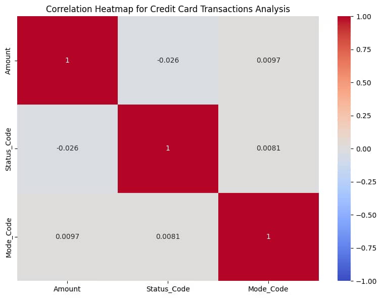
# Heatmap for correlation between Amount, Transaction_Status, and Payment_Mode
df_encoded = df.copy()
df_encoded['Transaction_Status_Code'] = df_encoded['Transaction_Status'].astype('category').cat.codes
df_encoded['Payment_Mode_Code'] = df_encoded['Payment_Mode'].astype('category').cat.codes
correlation_matrix = df_encoded[['Amount', 'Transaction_Status_Code', 'Payment_Mode_Code']].corr()
plt.figure(figsize=(8, 6))
sns.heatmap(correlation_matrix, annot=True, cmap='coolwarm', vmin=-1, vmax=1, square=True)
plt.title('Correlation Heatmap of Amount, Transaction Status, and Payment Mode', fontsize=14)
plt.tight_layout()
plt.show()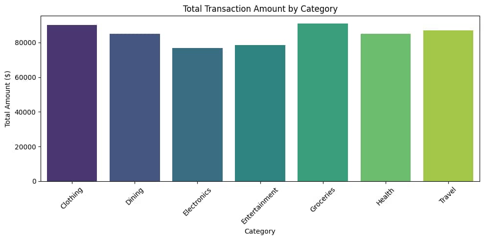
Explanation
- Bar Chart:
- Use Seaborn’s
barplotto visualize totalAmountbyCategory. - Customize with a
viridispalette, rotated x-labels, and clear titles for readability.
- Correlation Heatmap:
- Encode categorical variables (
Transaction_Status,Payment_Mode) as numerical codes usingcat.codes. - Compute the correlation matrix for
Amount,Transaction_Status_Code, andPayment_Mode_Code. - Use Seaborn’s
heatmapwithcoolwarmcmap to show correlations, with annotations for clarity.
Insights
- The bar chart highlights dominant categories, guiding resource allocation.
- The heatmap reveals relationships, e.g., if high amounts correlate with specific statuses, aiding risk assessment.
Key Findings
- Revenue Drivers: Categories like Electronics or Travel may dominate total spending, suggesting focus areas for promotions.
- Fraud Risks: High daily transactions, rapid location changes, and large online transactions are red flags for fraud.
- Customer Behavior: Age group analysis may show higher spending in certain demographics, e.g., >50 years.
- Payment Issues: High decline rates for specific payment modes indicate potential processing improvements.
Business Applications
- Fraud Prevention: Implement real-time alerts for high-risk patterns to reduce losses.
- Marketing Strategies: Target high-spending categories and age groups with tailored campaigns.
- Operational Improvements: Optimize payment processing for modes with high decline rates.
- Partnerships: Strengthen ties with top merchants to enhance customer offerings.
Conclusion
This guide simplifies credit card transactions analysis with Python, covering data cleaning, fraud detection, and visualization. By following these steps, you can uncover insights to drive financial decisions.